Efficient Filtering and Fitting of Models Derived from Integro-Difference Equations
Author
Evan Tate Paterson Hughes
1 Introduction
The Integro-Difference equation model (here abbreviated as IDEM 1) is dynamics-based spatio-temporal aiming to model diffusion and convection by making the value of a process a weighted average of it’s previous time, plus noise.
[NOTE: I intend to create a more thorough background for the introduction here.]
2 Integro-difference Based Dynamics
As common and widespread as the problem is, spatio-temporal modelling still presents a great deal of difficulty. Inherently, Spatio-Temporal datasets are almost always high-dimensional, and repeated observations are usually not possible.
Traditionally, the problem has been tackled by the moments (usually the means and covariances) of the process in order to make inference (Wikle, Zammit-Mangion, and Cressie (2019), for example, call this ‘descriptive’ modelling). While this method can be sufficient for many problems, there are many cases where we are underutilizing some knowledge of the underlying dynamic systems involved. For instance, in temperature models, we know that temperature has movement (convection) and spread (diffusion), and that the state at any given time will depend on its state at previous times 2. We call models which make use of this ‘dynamic’ models.
A general way of writing such hierarchical dynamical models might be
This describes the scalar random fields \(Z_t(\cdot), Y_t(\cdot)\in \mathbb R\) over the space \(\mathcal D\subset \mathcal R^d\), which are the observed data and unobserved dynamic process, respectively. \(\mathcal M_t\) here is a non-random ‘propagation operator’, defining how the process evolves with respect to it’s previous state(s), and \(\mathcal O_t\) is a non-random ‘observation operator’, defining how observations of a given process state are taken. Both these fields have random (usually time-independent) additive random fields, \(\omega_t(\cdot), \epsilon_t(\cdot)\), and we also include non-random measured linear covariate terms \(x(\cdot)^{\intercal}\bv \beta\).
If we discretize the space into \(n\) $spatial locations \(\{\bv s_i\}_{i=1,\dots, n}\), assume the operator are linear, assert a Markov condition, and assume the errors are all normal, we get a simple linear dynamic system;
where we have written \(\bv Y_t = (Y_t(\bv s_1),\dots, Y_t(\bv s_n))\), and similar for \(\bv Z_t, \bv \epsilon_t\) and \(\bv\omega_t\), and we have written \(\tilde{\bv Z}_t = \bv Z_t + X^{\intercal}\bv \beta\). This is a well-known type of system, the process \(Y\) can easily be estimated either directly of with a Kalman filter/smoother and variants, which will be discussed later.
However, this model is restrictive and high-dimensional; \(M_t\), the primary quantities which needs estimation, is of dimension \(n\times n\), of which there are \(T\) matrices to be estimated. Even if we allow the propagation matrix to be invariant in time, we can still only make predictions at the stations \(\{\bv s_i\}\).
This motivates a different approach; in particular, one which allows us to estimate the random field at arbitrary points \(Y_t(\bv s)\) using some spectral decomposition, which would alleviate these problems.
The Integro-difference equation model attempts to generalise Equation 1 into the continuous space by replacing the discrete linear \(M_t\) by a continuous integral equivalent;
Where \(\omega_t(\bv s)\) is a small scale gaussian variation with no temporal dynamics (Cressie and Wikle 2015 call this a ‘spatially descriptive’ component), \(\bv X(\bv s)\) are spatially varying covariates (for example, in a large-scale climate scenario, this might be latitude, concentration of some chemical/element like nitrogen) \(\kappa(\bv s, \bv r)\) is the driving ‘kernel’ function, and \(\epsilon_t\) is a Gaussian white noise ‘measurement error’ term.
Our operator is now \(\mathcal M(Y_t(\bv s)) = \int_{\mathcal D_s} \kappa_t(\bv s,\bv r) Y_t(\bv r) d\bv r\), which can model diffusion and convection by choosing the shape of \(\kappa\) (which, from now on, we will assume to be temporally invariant). This kernel defines how each point in space is affected by every other point in space at the previous time. For example, if we choose a Gaussian-like shape,
\[\begin{split}
\kappa(\bv s, \bv r; \bv m, a, b) = a \exp \left( -\frac{1}{b} \vert \bv s- \bv r +\bv m(\bv s)\vert^2 \right),
\end{split}
\]
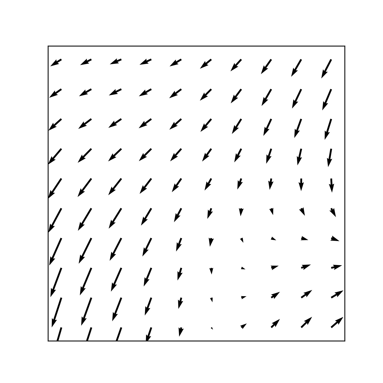
then the ‘flow’ would be in the direction of \(-\bv m(\bv s)\), and the diffusion would be controlled by \(b\) and \(a\). This creates a ‘spatially variant kernel’, where the direction of flow varies across the space, as in Figure 1.
Invariant Kernel Direction
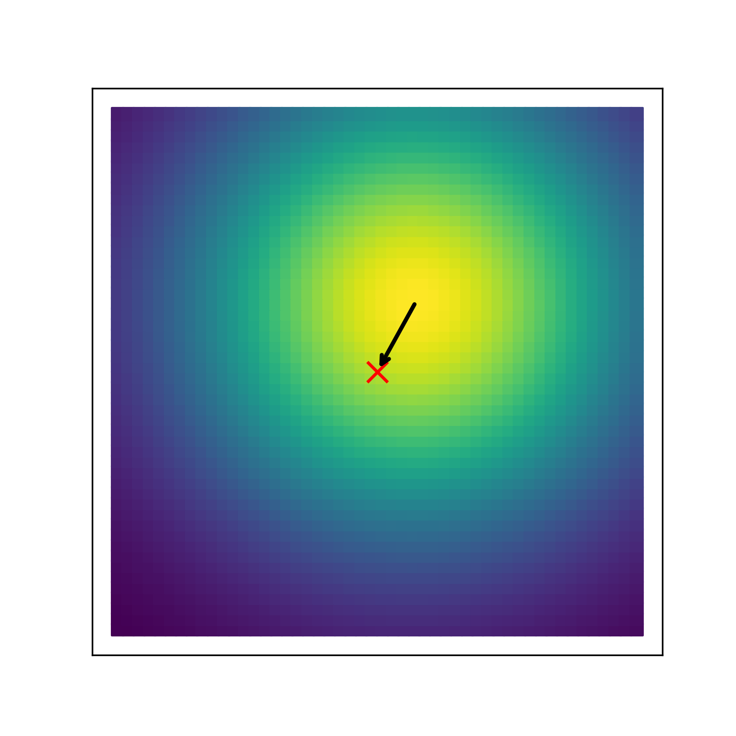
Invariant Kernel Strength
Figure 1: A spatially variant kernel across the region \([0,1]\times[0,1]\). The kernel direction is shown on the left, and on the right is the amount that each point affects the point \((0.5,0.5)\), marked with a red cross. ‘Flow’ is allowed to vary by a function \(\bv m(\bv s)\) which is chosen randomly using a basis expansion (see Section 3.3). The other two parameters are set at \(a=150,b=0.2\).
3 Spectral Representations
The key to being able to computationally work with IDEMs, as perhaps originally made by Wikle and Cressie (1999), is to work with the spectral decomposition of the process, in order to coerce the model hierarchy into a more familiar linear dynamical system form, like Equation 1.
This kind of dimension-reduction allows us to parametrise spatial fields with as few or as many parameters as we want.
3.1 Process decomposition
Choose a complete class of spatial spectral basis functions, \(\{\phi_i(\cdot): \mathcal D\to \mathbb R\}_{i=1,\dots}\), and decompose the process spatial field at each time;
where we truncate the expansion at some \(r\in\mathbb N\). Notice that we can write this in vector/matrix form, where we consider the vector field \(\bv \phi(\cdot) = (\phi_1(\cdot),\dots, \phi_r(\cdot))^\intercal\); considering times \(t=1,2,\dots, T\), we set
We can effectively now work exclusively with \(\bv \alpha_t = (\alpha_{1,t},\dots, \alpha_{r,t})^\intercal\). To do so, we need to find the evolution equation of \(\bv \alpha_t\), as given below.
Theorem 1 (Spectral form of the state evolution) Define the Gram matrix;
We then multiply both sides by \(\bv \phi(s)\) and integrate over \(\bv s\)
\[\begin{split}
\int_{\mathcal D_s} \bv\phi(\bv s)\bv\phi(\bv s)^{\intercal} d\bv s \bv\alpha_{t+1} &= \int\bv\phi(\bv s)\int \kappa(\bv s, \bv r)\bv\phi(\bv r)^\intercal d\bv r d \bv s\ \bv\alpha_t + \int \bv \phi(\bv s)\omega_t(s)d\bv s\\
\Psi \bv\alpha_{t+1} &= \int\int \bv\phi(\bv s)\kappa(\bv s, \bv r) \bv\phi(\bv r)^\intercal d\bv r d \bv s\ \bv\alpha_t + \int \bv \phi(\bv s)\omega_t(s)d\bv s.
\end{split}
\]
So, finally, pre-multipling by the inverse of the gram matrix, \(\Psi^{-1}\) (Equation 6), we arrive at the result.
3.2 Spectral form of the Process Noise
We still have to set out what the process noise, \(\omega_t(\bv s)\), and it’s spectral counterpart, \(\bv \eta_t\), are. Dewar, Scerri, and Kadirkamanathan (2008) fix the variance of \(\omega_t(\bv s)\) to be uniform and uncorrelated across space and time, with \(\omega_t(\bv s) \sim \mathcal N(0,\sigma^2)\) It is then easily shown that \(\bv\eta_t\) is also normal, with \(\bv\eta_t \sim \mathcal N(0, \sigma^2\Psi^{-1})\).
However, in practice, we simulate in the spectral domain; that is, if we want to keep things simple, it would make sense to specify (and fit) the distribution of \(\bv\eta_t\), and compute the variance of \(\omega_t(\bv s)\) if needed.
Lemma 1 Let \(\bv\eta_t \sim \mathcal N(0, \Sigma_\eta)\), and \(\cov[\bv\eta_t, \bv \eta_{t+\tau}] =0\), \(\forall \tau>0\). Then \(\omega_t(\bv s)\) has covariance
Since, once again, \(\mathbb E[\bv\omega_t(\bv s)]=0\).
For the \(\tau\neq0\) case, it is simple to show that the covariance is 0.
3.3 Kernel Parameterisations
Next is the part of the system, which defines the dynamics; the kernel function, \(\kappa\). There are a few ways to handle the kernel. One of the most obvious is to expand it out into a spectral decomposition as well;
This can allow for a wide range of interestingly shaped kernel functions, but see how these basis functions must now act on \(\mathbb R^2\times \mathbb R^2\); to get a wide enough space of possible functions, we would likely need many terms in the spectral expansion.
A much simpler approach would be to simply parametrise the kernel function, to \(\kappa(\bv s, \bv r, \bv \theta_\kappa)\). We then establish a simple shape for the kernel (e.g. Gaussian) and rely on very few parameters (for example, scale, shape, offsets). The example kernel used in the jaxidem is a Gaussian-shape kernel;
\[\kappa(\bv s, \bv r; \bv m, a, b) = a \exp \left( -\frac{1}{b} \vert \bv s- \bv r +\bv m\vert^2 \right).
\]
Of course, this kernel lacks spatial dependence. We can add spatial variance back by adding dependence on \(\bv s\) to the parameters, for example, varying the offset term as \(\bv m(\bv s)\). Of course, now we are back to having entire functions as parameters, but taking the spectral decomposition of the parameters we actually want to be spatially variant seems like a reasonable middle ground (Cressie and Wikle 2015). The actual parameters of such a spatially-variant kernel are then the spectral coefficients for the expansion of any spatially variant parameters, as well as any constant parameters. This is precisely what is plotting in Figure 1, where the spectral coefficients are randomly sampled from a multivariate normal distribution;
where \(m^{(x)}_i\) and \(m^{(y)}_i\) are coefficients for the x and y coordinates respectively, and \(\phi_{\kappa, i}(\bv s)\) are basis functions (e.g. bisquare 3) functions in Figure 1).
3.4 IDEM as a linear dynamical system
To summarise, we have taken a truncated spectral decomposition to write the Integro-difference equation model as a more traditional linear dynamical system form (Equation 7). All that is left is to include our observations in our system.
Lets assume that at each time \(t\) there are \(n_t\) observations at locations \(\bv s_{1,t},\dots, \bv s_{n_{t},t}\). We write the vector of the process at these points as \(\bv Y(t) = (Y(s_{1,t};t), \dots, Y(s_{n_{t},t};t))^\intercal\), and, in it’s expanded form \(\bv Y_t = \Phi_t \bv\alpha_t\), where \(\Phi \in \mathbb R^{r\times n_{t}}\) is
As in, for example, (Wikle and Cressie 1999), Equation 10 is now in a traditional enough form that the Kalman filter can be applied to filter and compute many necessary quantities for inference, including the marginal likelihood. We can use these quantities in either an EM algorithm or a Bayesian approach, or directly maximise the marginal data likelihood
We now move on to an example simulation of this kind of model using its spectral decomposition and jaxidem.
3.5 Example Simulation
We can now use the above to simulate easily from such models; once we have chosen the appropriate decompositions, we simply compute \(M\) and propagate \(\bv \alpha_t\) as we would when simulating any other linear dynamic system. We then use the spectral coefficients to generate \(Y_t(\bv s)\) and \(Z_t(\bv s)\) in the obvious way.
jaxidem implements this in the function sim_idem, or through the more user-friendly method idem.IDEM.simulate. An object of the IDEM class contains all the necessary information about basis decompositions, and the simulate methods calls simIDEM without compromising its jit-ability (although just-in-time computation obviously isn’t as important for simulation, the jit-ed function could save compile time if someone want to simulate from many models).
The gen_example_idem method creates a simple IDEM object without many required parameters;
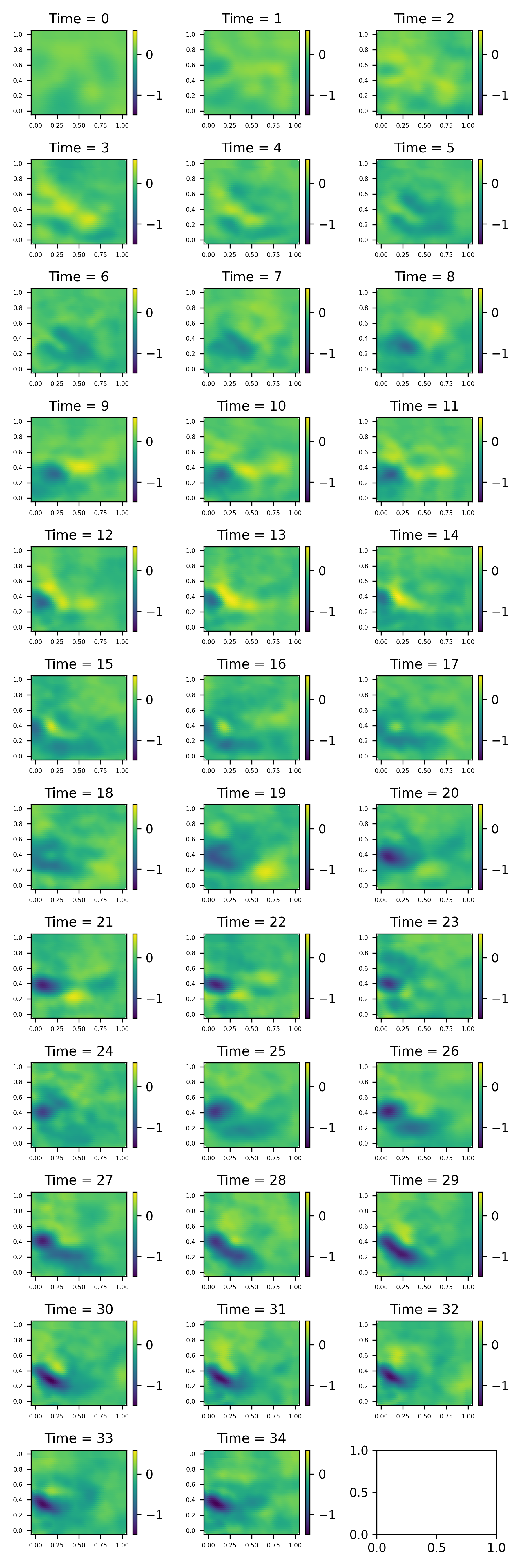
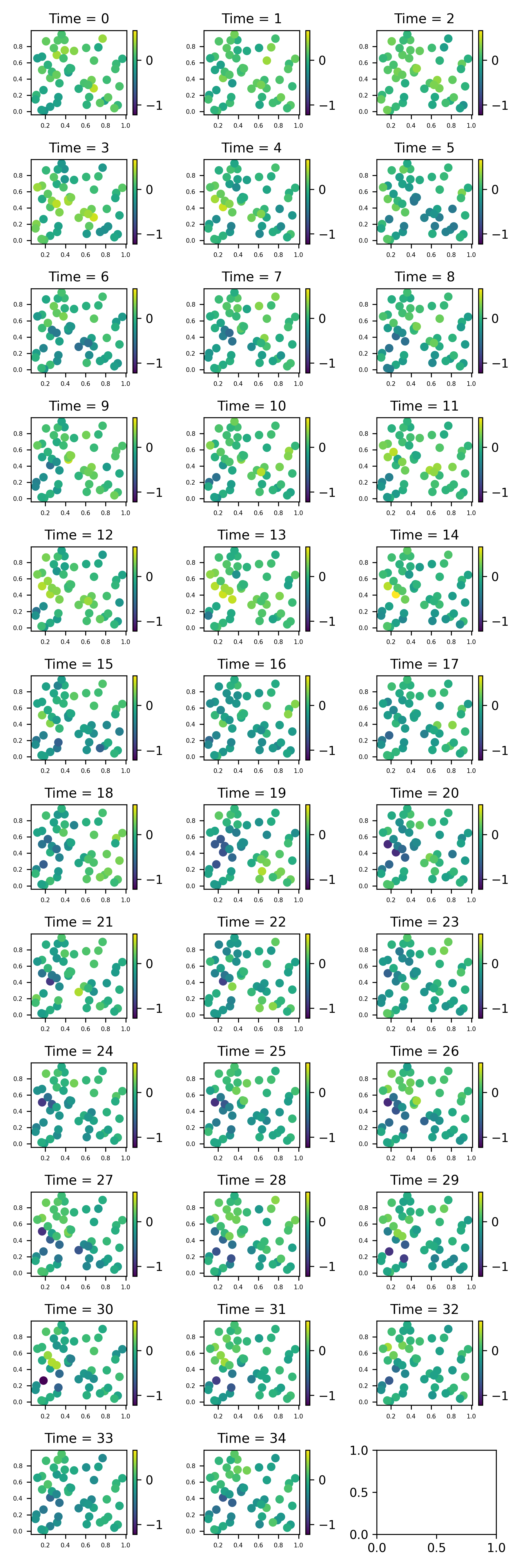
The resulting objects are of class st_data, containing a couple of niceties for handling spatio-temporal data, while still storing all data as JAX arrays. For example, the show_plot, save_plot and save_gif methods provide easy plotting;
Figure 2: Example simulations from an Integro-difference Equation Model. Kernel is generated with spatially varying flow terms, generated by bisquare basis functions with randomly generated coefficient. Note that some artefacts from the decomposition are visible, such as a faint chequerboard pattern in the process.
4 The Kalman filter, and its many flavours
The Kalman filter gives us linear estimates for the distribution of \(\bv\alpha_r\mid \{\bv Z_t=\bv z_t\}_{t=0,...,r}\) in any dynamical system like Equation 1. Now that we have written the IDEM in this form, this filter can now help compute estimates for the moments of the state \(\bv \alpha_t\). The Kalman filter also computes the marginal data likelihood, \(\pi(\{\bv z_t\}_{t=1,\dots, T}\mid \bv\theta)\), where \(\bv\theta\) are the model parameters. This allows us to perform maximum-likelihood estimation (as well as any other likelihood-based method of optimization). We will not prove the Kalman filter here, (for that, see, for example, Shumway, Stoffer, and Stoffer 2000).
Since it’s initial formulation in the 50s by a variety of authors (Kálmán included) there have been many variations of the Kalman filter proposed, even as recently as this decade with the temporally paralellised Kalman filter, more technically a variant of the information form of the Kalman filter, by Särkkä and Garcı́a-Fernández (2020).
For the initial terms, we choose Bayesian-like prior moments \(m_{0\mid0}=m_0\) and \(P_{0\mid0}=\Sigma_0\). For convenience and generality, we write \(\Sigma_\eta\) and \(\Sigma_\epsilon\) for the variance matrices of the process and observations. Note that, if the number of observations change at each time point (for example, due to missing data), then \(\Sigma_\epsilon\) should be time varying (even in its shape); we could either always keep it as uncorrelated so that \(\Sigma_\epsilon = \mathrm{diag} (\sigma_\epsilon^2)\), or perhaps put some kind of distance-dependant covariance function to it.
To move the filter forward, that is, given \(m_{t\mid t}\) and \(P_{t\mid t}\), to get \(m_{t+1\mid t+1}\) and \(P_{t+1\mid t+1}\), we first predict
\[\begin{split}
\bv m_{t+1\mid t} &= M \bv m_{t\mid t},\\
P_{t+1\mid t} &= M P_{t\mid t} M^\intercal + \Sigma_\eta,
\end{split}
\tag{11}\]
then we add our new information, update, with \(z_{t}\);
Starting with \(m_0\) and \(P_0\), we can then iteratively move across the data to eventually compute \(m_{T\mid T}\) and \(P_{T\mid T}\).
Assuming Gaussian all random variables here are Gaussian, this is the optimal mean-square estimators for these quantities, but even outside of the Gaussian case, these are optimal for the class of linear operators.
We can compute the marginal data likelihood alongside the Kalman filter using the prediction errors \(\bv e_t\). These, under the assumptions we have made about \(\bv \eta_t\) and \(\bv\epsilon_t\) being normal, are also normal with zero mean and variance
In some computational scenarios, it is beneficial to work with vectors of consistent dimension. In Python JAX, the efficient scan method works only with such arrays; JAX has no support for jagged arrays, and traditional for loops will likely lead to long compile times when jit-compiled. Although there are some tools in JAX to get around this problem (namely the jax.tree functions which allow mapping over PyTrees), scan is still a large problem; since the Kalman filter is, at it’s core, a scan-type operation (scanning over the data), this causes a large problem when the observation dimension is changing, as is frequent with many spatio-temporal data.
But it is possible to re-write the Kalman filter in a way which is compatible with this kind of data. The ‘information filter’ (sometimes called inverse Kalman filter or other names) involves transforming the data into its ‘information form’, which will always have consistent dimension, allowing us to avoid jagged scans.
The information filter is simply the Kalman filter re-written to use the Gaussian distribution’s canonical parameters 4, those being the information vector and the information matrix. If a Gaussian distribution has mean \(\bv\mu\) and variance matrix \(\Sigma\), then the corresponding information vector and information matrix is \(\nu = \Sigma^{-1}\mu\) and \(Q = \Sigma^{-1}\), correspondingly.
Theorem 2 The Kalman filter can be rewritten in information form as follows (for example, Khan 2005). Write
We can see that the information form of the observations (Equation 14) will always have the same dimension 5. For our purposes, this means that jax.lax.scan will work after we ‘informationify’ the data, which can be done using jax.tree.map. This is implemented in the functions information_filter and information_filter_indep (for uncorrelated errors).
There are other often cited advantages to filtering in this form. It can be quicker that the traditional form in certain cases, especially when the observation dimension is bigger than the state dimension (since you solve a smaller system of equations with \([S_t + \Sigma_\eta]^{-1}\) in the process dimension instead of \([\Phi_t P_{t+1\mid t} \Phi_t^\intercal + \Sigma_\epsilon]^{-1}\) in the observation dimension) (Assimakis, Adam, and Douladiris 2012).
The other often mentioned advantage is the ability to use a flat prior for \(\alpha_0\); that is, we can set \(Q_0\) as the zero matrix, without worrying about an infinite variance matrix. While this is indeed true, it is actually possible to do the same with the Kalman filter by doing the first step analytically, see Section 7.3.
As with the Kalman filter, it is also possible to get the data likelihood in-line as well. Again, we would like to stick with things in the state dimension, so working directly with the prediction errors \(\bv e_t\) should be avoided. Luckily, by multiplying the errors by \(\Phi_t^\intercal \Sigma_\epsilon^{-1}\), we can define the ‘information errors’ \(\bv \iota_t\);
In certain high-dimensional cases, the Kalman filter (and, indeed, the information filter) can encounter numerical stability issues. For example, in the predict step of the standard Kalman filter, note the update step for the variance matrix
Somewhat masked within this equation is two (often very small) variance matrices subtracted from eachother. While analytically, the result is still guaranteed to be positive (semi-)definite, when done in floating point arithmetic (especially in single-precision or lower), the result can often be numerically indefinite. When the variances are very low (as they often become in these Kalman filters), the eigenvalues come out very close to zero and can tick over to becoming negative erroneously. This can lead to definiteness issues with all the other variance matrices, most crucially \(\Sigma_t\)Equation 13. When this happens, computation of the likelihood likely fails (certainly when such a computation involves a Cholesky decomposition). Even if such is rare to happen with 64-bit precision, modern GPU hardware tends to be much more efficient with Single (32-bit) precision, so it may still be desirable to increase stability if it permits using a lower precision. The Square-root filter and the SVD filter are such algorithms.
4.3.1 The Square-root Kalman filter
The square-root Kalman filter has it’s origins soon after the standard Kalman filter gained popularity (Kaminski, Bryson, and Schmidt 1971). Of course, computational and memory constraints necessitated stable and memory-efficient approaches, while today the standard Kalman filter (and, more recently, it’s parallel counterpart, to be covered in section [TBD]) usually suffice.
As its name suggests, this variant involves carriyng through the square roots of variances 6 instead of the variances themselves. This leads to, at least in some sense, an increased precision, and we can always guarentee that, at least analytically, the square of these square roots (the variances) are positive (semi-)definite.
While the square root filter has been known for a long time (even used during NASA’s Apollo program), more recently, (Tracy 2022) wrote it neatly in terms of the QR decomposition, and this is what we base the presentation on here.
The key observation used for this filter is that if we have the sum of two equations where a square root is known for both, it can be written
\[\begin{split}
X + Y &= A^\intercal A + B^\intercal B\\
&= \left[A^\intercal\ B^\intercal\right] \left[\begin{matrix}A\\B\end{matrix}\right]
\end{split}
\]
Taking the QR decomposition of the vertical block yields QR, and since \((QR)^\intercal\ (QR) = R^\intercal Q^\intercal Q R = R^\intercal R\), so \(R\) is a square root of \(X+Y\). This motivates the following ‘QR operator’
Beginning with the Cholesky decomposition of the initial variances, \(P_0 = U_0^\intercal U_0\), \(\Sigma_{\eta} = U_{\eta}^\intercal U_{\eta}\) and \(\Sigma_\epsilon = U_{\epsilon}^\intercal U_{\epsilon}\) the predict step for the variance becomes
which is often simplified further to Equation 12, but as discussed that involves negation of two square root matrices; this form is more complicated and involves more matrix computation, but guarentees that the result will be positive (semi-)definite. Furthermore, this is also in a form that allows us to easily find the square root with the QR trick;
Of course, from here, we can similarily easily compute the data likelihood using \(U_{e,t+1}\), using standard techniques; the multivariate normal likelihood is usually computed using the cholesky decomposition of the variance matrix anyway. The result is an algorithm which is of a higher order than the standard Kalman filter, but the stability is often worth the comprimise. Once jit-compiled, the function sqrt_filter_indep on a moderately sized IDEM (on a discrete GPU) on 64-bit precision 7 takes approximately 23.5ms, compared to kalman_filter_indep taking approximately 7.8ms, achieving similar log-likelihoods (whith some difference due to precision). However, running the code in 32-bit causes the Kalman filter likelihood computation to fail, the square-root filter succeeds at a time of 7.0ms.
4.3.2 Square-root Information filter
Very similarily, we can write the information filter using the square roots of the information matrices. We will label roots of ‘information-type’ matrices with \(R\), and ‘variance-type’ matrices (their inverse) with \(U\).
We now carry the data’s information matrix’s (Equation 14) square root as well, \(R_t^{(I)} = \sqrt(\Phi_t^\intercal\Sigma_\epsilon^{-1} \Phi_t)\), with the same observation vector.
So, once again, beginning with the lower-triangular cholesky decomposition \(Q_0 = R^\intercal R\), and the upper-triangular \(\Sigma_{\eta} = U_{\eta}^\intercal U_{\eta}\) and \(\Sigma_\epsilon = U_{\epsilon}^\intercal U_{\epsilon}\).
So, to predict step for the information matrix (Equation 15) becomes
Beyond the filtering, another task is smoothing. That is, filters estimate \(\bv m_{T\mid T}\) and \(P_{T\mid T}\), but there is use for estimating \(\bv m_{t\mid T}\) and \(P_{t\mid T}\) for all \(t=0,\dots, T\).
We simply work backwards from \(\bv m_{T\mid T}\) and \(P_{T\mid T}\) values using what is known as the Rauch-Tung-Striebel (RTS) smoother;
We can clearly see, then, that it is crucial to keep the values in Equation 11.
We can then also compute the lag-one cross-covariance matrices \(P_{t,t-1\mid T}\) using the Lag-One Covariance Smoother. This will b useful, for example, in the expectation-maximisation algorithm later. From
These values can be used to implement the expectation-maximisation (EM) algorithm which will be introduced later.
5 EM Algorithm (NEEDS A LOT OF WORK, PROBABLY IGNORE FOR NOW)
Instead of the marginal data likelihood, we may instead want to work with the ‘full’ likelihood, including the unobserved process, \(l(\bv z(1),\dots, \bv z(T), \bv Y(1), \dots, \bv Y(T)\mid \bv\theta)\), or, equivalently, \(l(\bv z(1),\dots, \bv z(t), \bv \alpha(1), \dots, \bv\alpha(T)\mid \bv\theta)\). This is difficult to maximise directly, but can be done with the EM algorithm, consisting of two steps, which can be shown to always increase the full likelihood.
In the EM algorithm, we maximise the full likelihood by changing \(\bv \theta\) in order to increase (Equation 23), which can be shown to guarantee that the Likelihood \(L(\bv \theta)\) also increases. The idea is then that repeatedly alternating between adjusting \(\bv \theta\) to increase Equation 23, and then doing the filters and smoothers to obtain new values for \(\bv m_{t\mid T}\), \(P_{t\mid T}\), and \(P_{t,t-1\mid T}\).
6 Algorithm for Maximum Complete-data Likelihood estimation
Overall, our algorithm for Maximum Likelihood estimation is:
Set \(i=0\) and take an initial guess for the parameters we are considering, \(\bv\theta_0=\bv\theta_i\)
Starting from \(\bv m_{0\mid 0}=\bv m_0, P_{0\mid0}=\Sigma_0\), run the Kalman Filter to get \(\bv m_{t\mid t}\), \(P_{t\mid t}\), and \(K_t\) for all \(t\)Equation 12,
Starting from \(\bv m_{T\mid T}, P_{T\mid T}\), run the Kalman Smoother to get \(\bv m_{t\mid T}\), \(P_{t\mid T}\), and \(J_t\) for all \(t\) (Equation 20),
Starting from \(P_{T,T-1\mid T} = (I - K_nA_n) MP_{T-1\mid T-1}\), run the Lag-One Smoother to get \(\bv m_{t,t-1\mid T}\) and \(P_{t,t-1\mid T}\) for all \(t\)Equation 21,
Use the above values to construct \(\mathcal Q(\bv\theta;\bv \theta')\) in Equation 23,
Maximise the function \(\mathcal Q(\bv\theta;\bv \theta')\) to get a new guess \(\bv \theta_{i+1}\), then return to step 2,
Stop once a certain criteria is met.
7 Appendix
7.1 Woodbury’s identity
The following two sections will make heavy use of the Woodbury identity.
Lemma 2 (Woodbury’s Identity) We have, for conformable matrices \(A, U, C, V\),
\[\begin{split}
(A + UCV)^{-1} = A^{-1} - A^{-1} U (C^{-1} + VA^{-1}U)^{-1}VA^{-1}.
\end{split}
\tag{24}\]
Proof. Firstly, for the prediction step, using \(S_t = M^{-\intercal}Q_{t\mid t}M^{-1}\) and \(J_t = S_t(\Sigma_\eta^{-1} + S_t)^{-1}\) and the identities Equation 24 and Equation 25,
and now noting that \(\bv\nu_{t+1\mid t+1} = (Q_{t+1\mid t} + I_{t+1}) \bv m_{t+1\mid t+1}\), we complete the proof.
7.3 Truly Vague Prior with the Kalman Filter
It has been stated before that one of the large advantages of the information filter is the ability to use a completely vague prior \(Q_{0}=0\). While this is true, it is actually possible to do this in the Kalman filter by ‘skipping’ the first step (contrary to some sources, such as the Wikipedia page as of January 2025).
Theorem 3 In the Kalman Filter (Section 4.1), if we allow \(P_{0}^{-1} = 0\), effectively setting infinite variance, and assuming the propagator matrix \(M\) is invertible, we have
It is worth noting that (Equation 26) seems to make a lot of sense; namely, we expect the estimate for \(\bv m_0\) to look like a correlated least squares-type estimator like this.
References
Assimakis, Nicholas, Maria Adam, and Anargyros Douladiris. 2012. “Information Filter and Kalman Filter Comparison: Selection of the Faster Filter.” In Information Engineering, 2:1–5. 1.
Cressie, Noel, and Christopher K Wikle. 2015. Statistics for Spatio-Temporal Data. John Wiley & Sons.
Dewar, Michael, Kenneth Scerri, and Visakan Kadirkamanathan. 2008. “Data-Driven Spatio-Temporal Modeling Using the Integro-Difference Equation.”IEEE Transactions on Signal Processing 57 (1): 83–91.
Kaminski, Paul, Arthur Bryson, and Stanley Schmidt. 1971. “Discrete Square Root Filtering: A Survey of Current Techniques.”IEEE Transactions on Automatic Control 16 (6): 727–36.
Khan, Mohammad Emtiyaz. 2005. “Matrix Inversion Lemma and Information Filter.”Honeywell Techonology Solutions Lab, Bangalore, India.
Liu, Xiao, Kyongmin Yeo, and Siyuan Lu. 2022. “Statistical Modeling for Spatio-Temporal Data from Stochastic Convection-Diffusion Processes.”Journal of the American Statistical Association 117 (539): 1482–99.
Särkkä, Simo, and Ángel F Garcı́a-Fernández. 2020. “Temporal Parallelization of Bayesian Smoothers.”IEEE Transactions on Automatic Control 66 (1): 299–306.
Shumway, Robert H, David S Stoffer, and David S Stoffer. 2000. Time Series Analysis and Its Applications. Vol. 3. Springer.
Tracy, Kevin. 2022. “A Square-Root Kalman Filter Using Only QR Decompositions.”arXiv Preprint arXiv:2208.06452.
Wikle, Christopher K, and Noel Cressie. 1999. “A Dimension-Reduced Approach to Space-Time Kalman Filtering.”Biometrika 86 (4): 815–29.
Wikle, Christopher K, Andrew Zammit-Mangion, and Noel Cressie. 2019. Spatio-Temporal Statistics with r. CRC Press.
Footnotes
Historically, this has been abbreviated as IDE. However, with that abbreviation almost universally meaning ‘Integrated Development Environment’, here, we choose to include the ‘M’ in the abbreviation.↩︎
at least, in a discrete-time scenario. Integro-difference based mechanics can be derived from continuous-time convection-diffusion processes, see Liu, Yeo, and Lu (2022)↩︎
The bisquare functions, here, \(\phi_i(\bv s) = [1-\frac{\Vert \bv s - \bv c_i \Vert}{w_i}]^2 \cdot I(\Vert \bv s - \bv c_i \Vert < w_i)\) for \(i\) ‘centroids’ or ‘knots’, \(\bv c_i\in \mathcal D\), each with ‘radius’ \(w_i\)↩︎
that is, the parameters of the Gaussian distribution in it’s exponential family form↩︎
that being the process dimension, previously labelled \(r\), the number of basis functions used in the expansion of the process↩︎
A matrix \(A\) is said to be a ‘square root’ of a positive-definate matrix \(X\) if \(A^\intercal A = X\). Note that these square roots are not unique, but can be ‘rotated’ by an arbitrary unitary matrix. The ‘canonical’ square root is the Cholesky factor, the unique upper (or occasionally lower) triangular square root. This can be found for arbitraty square roots by taking the QR decomposition (or RQ decomposition), which effectively computes the upper-triangular square root, \(R\), and the unitary transformation \(Q^\intercal\) necessary to get there.↩︎