import jax
jax.config.update("jax_enable_x64", True)
import os
import jax.numpy as jnp
import jax.random as rand
import pandas as pd
import jaxidem.idem as idem
import jaxidem.utils as utils
import matplotlib.pyplot as plt

radar_df = pd.read_csv('data/radar_df.csv')Sydney Radar Data
1 The Sydney Radar Data Set
This is a data set… [more information here and plotting here]
2 Importing the relevant packages and Loading the data
Firstly, we load the relevant libraries and import the data.
We should put this data into jax-idems st_data type;
radar_data = utils.pd_to_st(radar_df, 's2', 's1', 'time', 'z') 2.1 Plotting the data
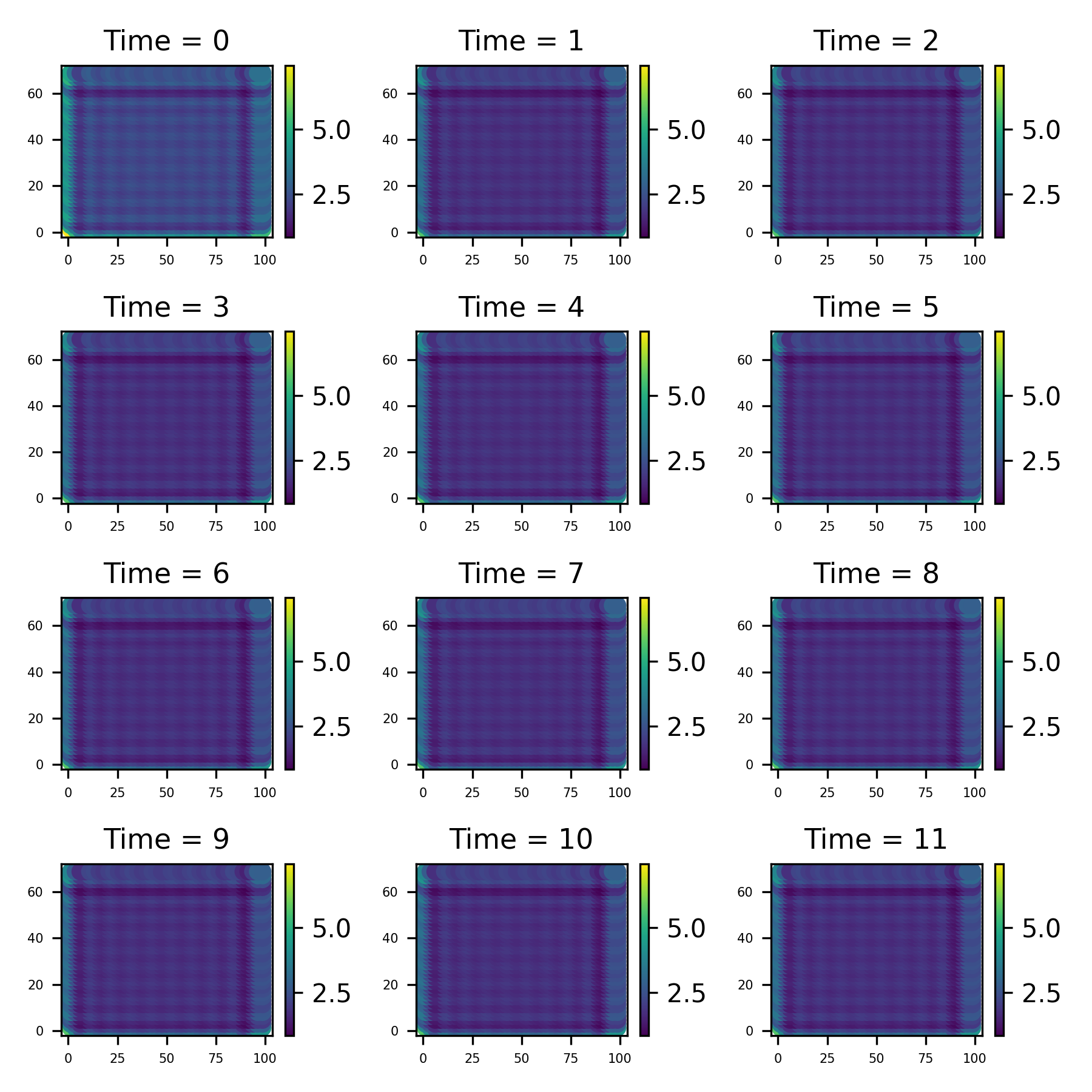
Firstly, lets take a look at the data set. I is a collection of 12 images taken at evenly spaced intervals. We can use the method st_data.show_plot to uickly make a plot of data like this;
radar_data.save_plot('figure/Sydney_plot.png')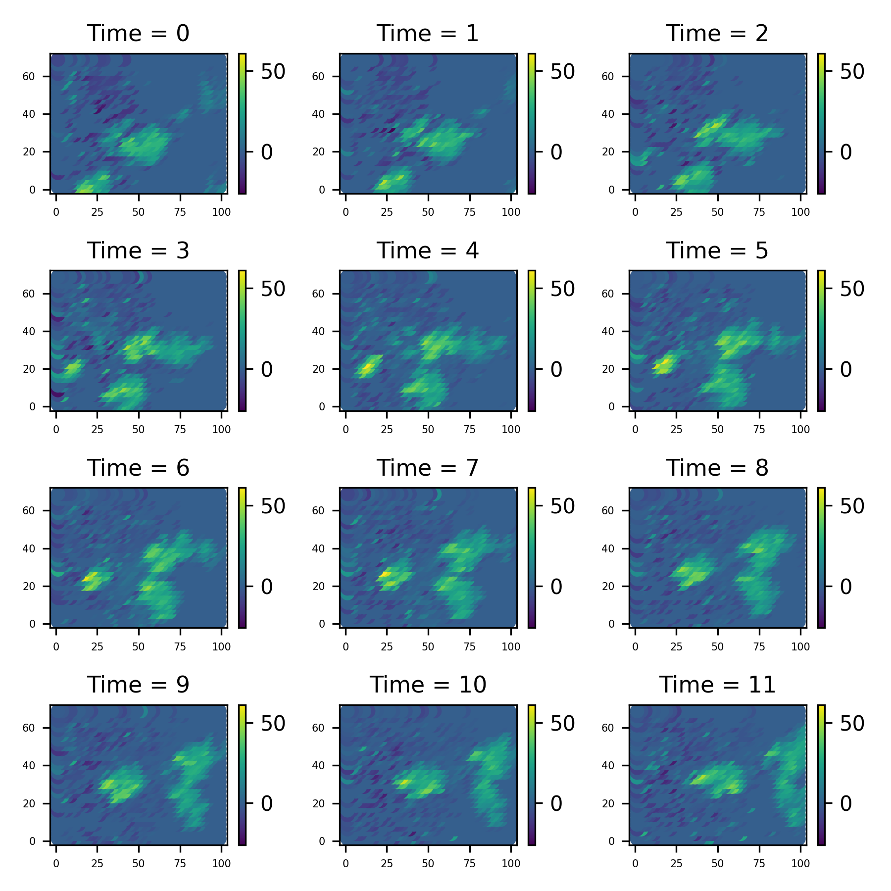
2.2 Modelling
We will firstly censor the data, so that we can assess the ‘blanks’ we filled in.
# Censor the data!
radar_df_censored = radar_df
# remove the final time measurements (for forecast testing)
radar_df_censored = radar_df_censored[radar_df_censored['time'] != "2000-11-03 08:45:00"]
# remove the a specific time (for intracast testing)
radar_df_censored = radar_df_censored[radar_df_censored['time'] != "2000-11-03 10:15:00"]
# three randomly chose indices ('dead pixels')
import numpy as np
np.random.seed(42) # reproducibility (jax.random is used elsewhere)
random_indices = np.random.choice(radar_df_censored.index, size=300, replace=False)
radar_df_censored = radar_df_censored.drop(random_indices)


# no covariates (besides intercept)
radar_data = utils.pd_to_st(radar_df_censored, 's2', 's1', 'time', 'z')
We now create an initial model for this data
model = idem.init_model(data=radar_data)This, by default, creates an invariant kernel model with no covariates beside an intercept, with cosine basis function for the process decomposition. We can now get the marginal data likelihood function of this model with the get_log_like method;
log_marginal = model.get_log_like(radar_data, method="sqinf", likelihood='partial')We can then use this function to do various inference techniques, like direclty maximising it or Bayesian MCMC methods. It is auto-differentiation compatible, so can easily be dropped into packages like optax or blackjax for these purposes.
The function takes, as an input, an object of type IdemParams, which is a NamedTuple containing the log variances, (transformed) kernel parameters, and the regression coefficients. The Model class has a value of these paramters, Model.params, and a method is provided to print these parameters in a clear way;
idem.print_params(model.params)Parameters:
sigma2_eps: 49.885520232669876
sigma2_eta: 49.885520232669876
Kernel Parameters:
Scale: [149.99999999999997]
Shape: [1.35]
Offset X: [0.0]
Offset Y: [0.0]
beta: [0.0]2.3 Maximum Likelihood Estimation
Once we have this marginal likelihood, there are a few ways to progress. A good start is with a maximum likelihood method. Obviously, we can no just take this lgo marginal function and maximise it in any way we see fit, but jaxidem.Model has a built-in method for this, Model.fit_mle. Given data, this will use a method from ‘optax’ to create a new output model with the fitted parameters.
import optax


fit_model_mle, mle_params = model.fit_mle(radar_data,
                                          optimizer = optax.adam(1e-2),
                                          max_its = 100,
                                          method = 'sqinf')
The resulting parameters are then
idem.print_params(mle_params)Parameters:
sigma2_eps: 5.723726749420166
sigma2_eta: 28.2664737701416
Kernel Parameters:
Scale: [0.08538345247507095]
Shape: [3.7510576248168945]
Offset X: [-5.437947750091553]
Offset Y: [-1.7626336812973022]
beta: [0.42389795184135437]Of course, we can use any other method to maximise this, by using whatever method desired on the function returned from Model.get_log_liklehood. We can update the model with new parameters using the method Model.update, and utils.flatten_and_unflatten (see documentation) allows working with flat arrays instead of PyTrees if needed.
2.4 Posterior Sampling
It is obviously desirable to use MCMC methods in order to sample from the posterior distribution. This can be done manually using the log likelihood, or by using the method Model.sample_posterior. We need to provide it with a sampling kernel; that is, a method to get from one state to the next.
2.5 Using Blackjax
From there, it is easy to sample from the posterior
key = jax.random.PRNGKey(1) # PRNG key
inverse_mass_matrix = jnp.ones(model.nparams)
num_integration_steps = 10
step_size = 1e-5
sample, _ = model.sample_posterior(key,
                                   n=10,
                                   burnin=0,
                                   obs_data=radar_data,
                                   X_obs=[X_obs for _ in range(T)],
                                   inverse_mass_matrix=inverse_mass_matrix,
                                   num_integration_steps=num_integration_steps,
                                   step_size = step_size,
                                   likelihood_method="sqinf",)
num_params = sample.shape[1]
fig, axes = plt.subplots(num_params, 1, figsize=(10, 10), sharex=True)
for i in range(num_params):
axes[i].plot(sample[:, i], lw=0.8, color='b')
axes[i].set_ylabel('')
axes[i].grid(True)
axes[-1].set_xlabel('Iteration')
fig.suptitle('Trace Plots', fontsize=16, y=0.95)
plt.tight_layout(rect=[0, 0, 1, 0.96])
plt.savefig('figure/hmc_trace.png')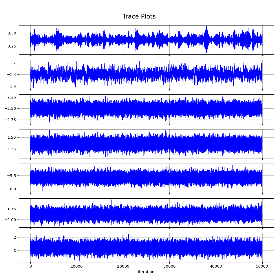
Lets take the posterior mean for some filtering and predicting.
# gets the function used to go from a flat array to a parameter of the type used in the models
fparams, unflatten = utils.flatten_and_unflatten(model.params)

post_mean = jnp.mean(sample, axis=0)
new_params = unflatten(post_mean)

new_model = model.update(new_params)

filt_data, filt_results = new_model.filter(radar_data, forecast = 3, method="kalman")filt_data.save_plot('figure/filtered_plot.png')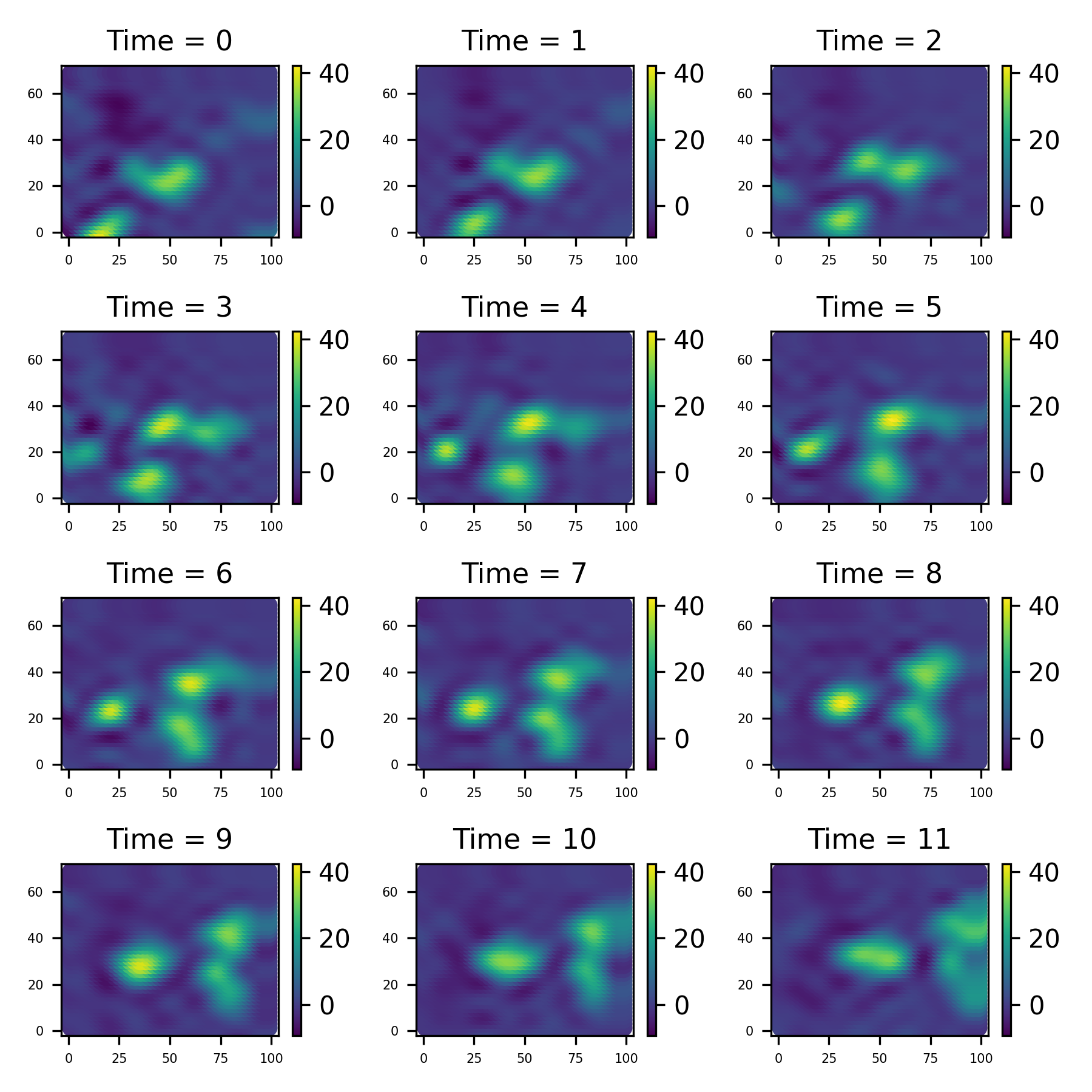
We’ve also forecasted the next 3 time points, and we can get them like this
#nuforecast = filt_results['nuforecast']
#Rforecast = filt_results['Rforecast']
#
#from jax.scipy.linalg import solve_triangular as st

#mforecast = st(Rforecast, nuforecast[..., None]).squeeze(-1)

mforecast = jnp.vstack((filt_results['ms'], filt_results['mforecast']))

# will build this in to the Model.filter method soon!
fore_data = idem.basis_params_to_st_data(mforecast, model.process_basis, model.process_grid)fore_data.save_plot('figure/fore_plot.png')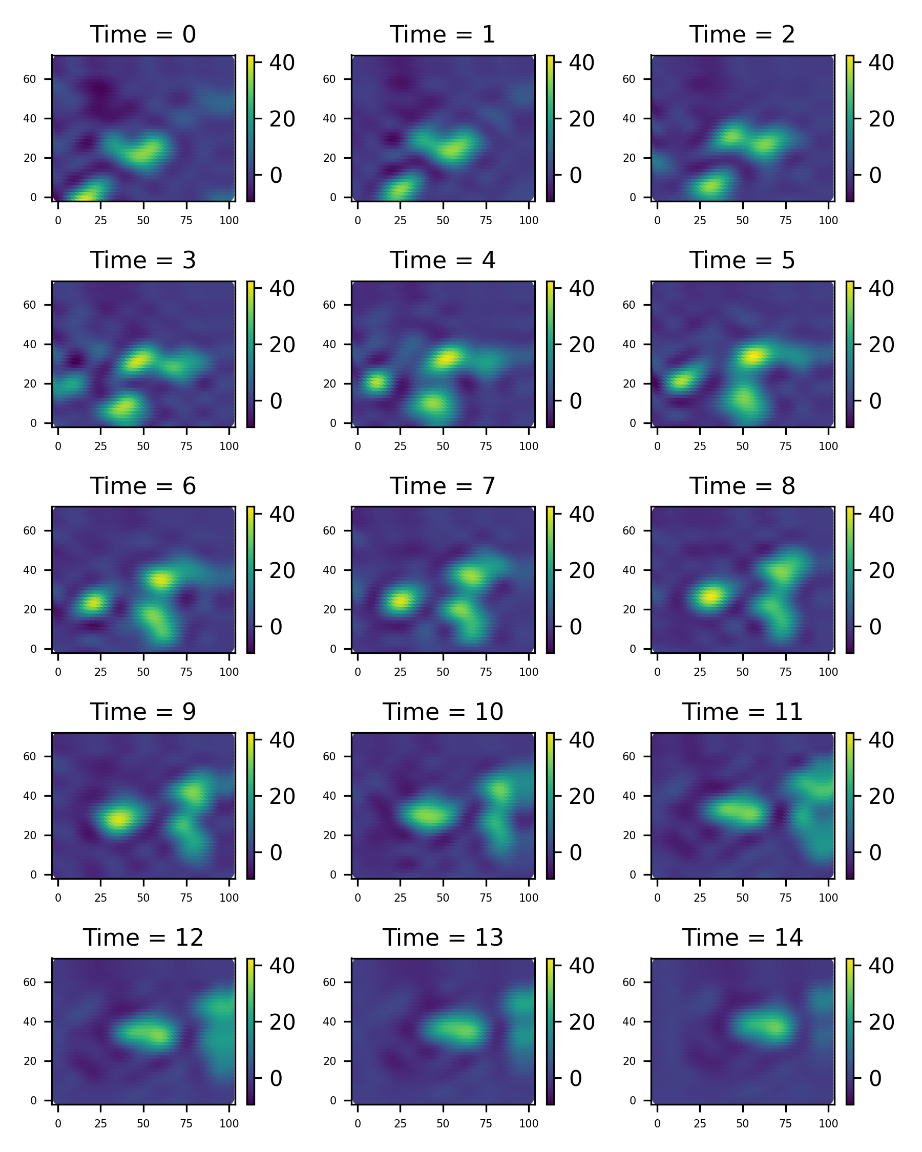
We can also plot the variances computed in the Kalman filter
Ps = filt_results['Ps']
Pforecast = filt_results['Pforecast']
combined = jnp.concatenate([Ps])#, Pforecast])

PHI = model.PHI_proc

process_variances = PHI @ combined @ PHI.T

marginals = jnp.diagonal(process_variances, axis1=1, axis2=2)

T = marginals.shape[0]

coords = jnp.concatenate([model.process_grid.coords for _ in range(T)])
times = jnp.repeat(jnp.arange(T), model.process_grid.coords.shape[0])
var_data = utils.st_data(x=coords[:, 0], y=coords[:, 1], times=times, z=marginals.ravel())var_data.save_plot('figure/var_plot.png')